Draw a Roche lobe diagram
Draw both Roche lobes, two detached levels and a contact envelope as vector outlines.
Use the same fill-out factor for both components at each level, and section_envelope() to leave out the contact envelope's watershed cut:
>>> import matplotlib.pyplot as plt
>>> import rocheometry
>>> from rocheometry.matplotlib import path_patch
>>>
>>> binary = rocheometry.BinaryGeometry(q=2.0)
>>> paths = []
>>> for component in (binary.component(1), binary.component(2)):
...     paths.append(component.lobe().section())
...     for factor in (-3.0, -1.0):  # detached
...         paths.append(component.surface(fill_out_factor=factor).section())
...     paths.append(component.surface(fill_out_factor=0.5).section_envelope())
>>> fig, ax = plt.subplots()
>>> for path in paths:
...     _ = ax.add_patch(path_patch(path, linewidth=1))
>>> for name, point in {"L1": binary.l1(), "L2": binary.l2(), "L3": binary.l3()}.items():
...     x, y, _ = point.position
...     _ = ax.plot(x, y, "+", color="black")
...     _ = ax.annotate(name, (x, y), xytext=(0, 6), textcoords="offset points")
>>> _ = ax.set(xlim=(-1.3, 1.9), ylim=(-0.7, 0.7), aspect="equal")
>>> plt.close(fig)
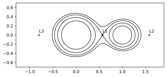
The same paths make a standalone SVG, with one <path> per outline:
>>> from rocheometry.svg import document_paths
>>> svg = document_paths(paths, y_axis="up")
>>> svg.count("<path")
8
The paths preserve their cubic Bézier segments when plotted or exported, so they stay sharp at any zoom. They approximate the sections to the outline accuracy bound. Selected levels must lie above L2, with fill-out factors below 1; see the model's scope. To include level curves beyond L2, draw a Roche potential diagram.